GUI building with plt


Over the years I have created dozens of GUIs using Matlab, nearly all of which involved collecting and/or viewing data and interacting with the data or data collection process in some way, and I suspect the same is true for the GUIs that you need to create. The first GUIs I created were quite difficult, but as I built up my bag of tools each new program became easier and quicker to write. The key I found was to avoid re-inventing the wheel each time and the best way to do that was to create a series of "pseudo objects". A pseudo object is a collection of Matlab graphics objects embedded with features commonly needed in Matlab GUI applications. (I chose to call them pseudo objects to distinguish them from the graphics objects supplied in the standard Matlab environment.) These pseudo objects are combined into one file exchange submission called pltSig (or sometimes shortened to plt for historical reasons). My primary goal is to make building GUI applications in Matlab easier, faster, and more fun while enabling you to create clearer, more concise code that is compatible across all Matlab platforms and versions.

The two main tasks in creating a GUI application are:
  1. Choosing the graphical elements and configuring the sizes and positions of these elements.
  2. Writing the code that enables these graphical elements to serve their intended purpose.
Matlab's GUI building tools (App Designer since 2016 and Guide for older Matlab versions) helps a lot with the first task but contributes little to the second. However, I've found that for all but the most trivial applications, the second task takes the most effort by far. My strategy is to aid the second task by providing a rich set of pseudo objects mentioned above. It may seem like this is a tall order for these new objects, but I hope the examples that follow will convince you that they can impressively reduce the amount of code you need to write. The pseudo-object idea is persuasive and once exposed to it you may find yourself inspired to create your own.

A parallel goal is to make it easier to learn Matlab GUI programming by providing many well-commented examples that demonstrate the use of all the pseudo objects. It's easier to begin a new GUI application by starting with an example that has at least some of the graphical features that you need. To this end, plt includes 37 application programs and demos covering a wide variety of GUI features and programming techniques. Although the standard Matlab plotting and graphical elements are thoroughly documented, a common complaint is that this information is spread out over thousands of pages of Matlab documentation making it difficult to find what you are looking for. Also, it is difficult to find examples for most features. This inspired me to design the plt help file to avoid these pitfalls by organizing plt's many features into one coherent help file including many examples. Every question from a plt user leads me to reexamine the documentation to see if I have described each feature and example as completely and clearly as possible.

Although the first task mentioned above (configuring sizes and positions of graphical elements) is not where most of the time is spent, without an appropriate tool this could be a painstaking task. Matlab's App Designer provides a reasonable solution to this problem however I found several annoyances with this tool:
  1. App Designer forces me to adopt a particular programming methodology and style. Although plt offers unique pseudo objects you are free to use all or none of them to suit your purpose and no demands are made on your programming style.
  2. App Designer saves all the work into a proprietary file format (.mlapp) that can only be viewed or modified by App Designer which makes me feel that I have lost control. GUI creation using the plt tools however saves everything as standard .m text files that can be edited with Matlab's editor or with your favorite programmer's editor.
  3. An App Designer GUI can only be run on the version of Matlab that you have (or newer). While using the plt GUI creation tools, one can create applications that can run on any Matlab version going all the way back to Matlab 6.1 (released in 2001)
  4. And most importantly App Designer is not compatible with the powerful pseudo objects that I have created.
As you will see from the examples below, the procedure for object positioning using the plt GUI tools are not quite as automated as App Designer, but I think it strikes a good balance between automation, power, and flexibility.

Since the pseudo objects are the key innovation that simplifies Matlab GUI programming, let's briefly summarize the ten pseudo objects that have been implemented so far: A more complete description of these pseudo objects from a programming perspective can be found here: Pseudo objects.

Now you are prepared to dive into the examples that follow:

A first example (gui1.m)

Our first GUI example doesn't do any plotting or anything useful for that matter, so it's not a very interesting program ... however, the code is very short and simple, giving you a chance to see how to use plt GUI tools with little effort.

I find that it is best to start working on a new GUI with pencil and paper. Imagine the control types and arrangement for the application and then sketch a mock-up such as this. Your finished application may not look like your first sketch, but with the rapid prototyping possible with Matlab and plt you can quickly iterate improvements in form, concept, and implementation.

Here I have decided on 3 pseudo sliders across the top followed below by a pseudo pop and a radio button on the left as well as a frame on the right containing 4 uicontrols (a popup, slider, button, and checkbox).

The bottom part of the GUI consists of two large objects for displaying lists of numbers. On the right is a simple text box with room to show about 10 lines of text. On the left is a listbox, which by virtue of its scroll bar can display a far larger data set (80 lines of text in this example).

The figure window is created in the first line of code. I decided to use a figure window 430 pixels wide and 350 pixels high, although this is just a guess and can be easily modified later. The menu bar is not needed for such a simple GUI so the menu property is set to 'none'. I chose a dark blue-green for the figure background:
function gui1()
  figure('name','gui1','menu','none','pos',[90 90 430 350],'color',[0 .3 .2]);
The next line defines the choices for the popup menu, and the line after that creates a cell array containing the positions for each of our twelve objects (Three pseudo sliders, a pseudo popup, a pseudo box (frame), and seven uicontrols):
  cho = {'choice A' 'choice B' 'choice C'}; % choices for popup control
  p = arrange(12);
The positions created by arrange are essentially haphazard and will have no relation to the final positions of the objects. This may seem a strange way to design a GUI, but it turns out to be a waste of time typing in position coordinates for the 12 objects when we will end up changing them anyway. This is a fast way to get started. Next, we create our 12 objects by calling plt for the pseudo objects and by calling uicontrol for the standard objects. We collect the handles of the object into vector h:

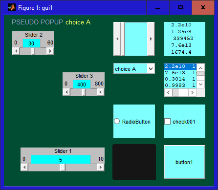
  h = [plt('slider',p{1}, 10,'Slider 1',@CBsli);
       plt('slider',p{2}, 60,'Slider 2',@CBsli);
       plt('slider',p{3},800,'Slider 3',@CBsli);
       plt('pop',p{4},cho,'disp("pseudo popup")','label','PSEUDO POPUP');
       plt('box',p{5});
       uicontrol('Style','radio',   'backgr',[.5 1 1],     'units','norm','pos',p{6},...
                                    'String','RadioButton','Callback',@CB);
       uicontrol('Style','popup',   'backgr',[.5 1 1],     'units','norm','pos',p{7},...
                                    'String', cho,         'Callback',@CB);
       uicontrol('Style','slider',  'backgr',[.5 1 1],     'units','norm','pos',p{8},...
                                    'String','slider',     'Callback',@CBsli);
       uicontrol('Style','pushb',   'backgr',[.5 1 1],     'units','norm','pos',p{9},...
                                    'String','button1',    'Callback',@CB);
       uicontrol('Style','checkbox','backgr',[.5 1 1],     'units','norm','pos',p{10},...
                                    'String','check001',   'Callback',@CB);
       uicontrol('Style','listbox', 'backgr',[.5 1 1],     'units','norm','pos',p{11});
       uicontrol('Style','text',    'backgr',[.5 1 1],     'units','norm','pos',p{12})];
The code above (in blue) is straightforward and will be the preferred style for many of you. Some of you may prefer more compact code (which I find easier to read), so what follows is the code that I actually included in gui1.m:

  h = [plt('slider',p(1:3),{10 60 800},{'Slider 1' 'Slider 2' 'Slider 3'},@CBsli);
       plt('pop',p{4},cho,'disp("pseudo popup")','label','PSEUDO POPUP');
       plt('box',p{5});
       uic('Style', {'radio'      'popup' 'slider' 'pushb'   'checkbox' 'listbox' 'text'},...
           'String',{'RadioButton' cho    'slider' 'button1' 'check001' ''        ''    },...
           'Callb', { @CB          @CB     @CBsli   @CB       @CB       ''        ''    },...
           'backgr',[.5 1 1],'units','norm','Pos',p(6:end))];
Note that the first three lines have been collapsed into one, since plt can create multiple pseudo objects with a single command. Also, the last 12 lines that create the 7 uicontrols has been collapsed onto 4 lines by using uic (which is similar to uicontrol except that it allows multiple controls to be created with a single command). There is nothing wrong with either style and which one you choose is largely a matter of taste. The workings of uic should be reasonably clear from this example, but you can see the details of this command (as well as the arrange command used above) in the Auxiliary functions section. And finally, the last line of the gui1 function:

  set(gcf,'user',h);  CBsli; % save the handles for the slider callback and execute it

We finish up by writing the control callbacks. The first four callbacks just send a message to the command window so you know that the callback has been executed. The last one (the slider callback) is the only one that does something, which is to update the data tables with new random data. Note that the random numbers are converted to strings using prin a substitute for sprintf that includes features commonly needed in GUI programming. To see the full documentation for prin simply type prin with no arguments into the command window.

function CB(a,b)        % default uicontrol callback ---------------
  disp(get(a,'style')); % display the uicontrol style

function CBsli(a,b)           % The slider callback ------------
  h = get(gcf,'user');        % Get the handle list
  r = 1e20.^(rand(3,80))/1e6; % generate some random numbers
  % Use the same random table of numbers for both the listbox and the textbox
  set(h(11:12),'string',prin('3{%6V  }~, ',r),'fontname','courier');


Now that we are done with the coding (just 18 lines of code!), start the GUI by typing gui1 in the command window. The figure window on the left will appear. You will see that the program is functional, and the callbacks get executed as expected. However, the control placement looks nothing like our sketch. We are about to fix that.

Type plt move in the command window to enable the mouse-driven repositioning mode. To indicate that the repositioning mode is active, plt will gray out the graphical objects, indicating that the object callbacks have been disabled. Now we can:

        left-click, hold, and drag to move an object.
        right-click, hold and drag to resizes an object.
        Double click to open an object's property inspector window.

Now use the mouse to resize and position the objects to match your sketch, or until the arrangement pleases you. (BTW, when moving the pseudo popup, drag the "choice A", not the popup's label in capital letters.) Then click on each object once in the order they are defined in the h array. As you do this you will see something like the following text appears in the command window:

sli: 401  .020 .920 .300     ;  % Slider 1
sli: 406  .350 .920 .300     ;  % Slider 2
sli: 411  .680 .920 .300     ;  % Slider 3
pop: 101  .270 .500 .250 .200;  % choice A
axi:  51  .540 .500 .440 .280;  % axes
uic: 207  .030 .560 .200 .060;  % RadioButton
uic: 206  .680 .710 .170 .050;  % choice A
uic: 205  .570 .610 .380 .060;  % slider
uic: 204  .570 .520 .170 .060;  % button1
uic: 203  .780 .520 .170 .060;  % check001
uic: 202  .015 .040 .500 .410;  % 2.40e7  10098.  .02290 
uic: 201  .540 .040 .440 .410;  % 2.40e7  10098.  .02290 
Copy this text from the command window and paste it into your editor, right after the arrange command. (Now we can close the gui1 figure, as it has served its purpose). The first column is a three-letter identifier for the object type. The native Matlab types - uicontrol, uitable, uipanel, axis, and text are identified as uic, uit, uip, axi, txt respectively and plt's pseudo objects are identified as sli, edi, pop, and xy. (xy refers to elements created by the cursor and plot pseudo objects.) The next column is a unique integer associated with the object. We won't need either of these columns this time, so we can simply delete those two columns, which can be done most quickly by using the column mode of your editor. (In example 2 below, we will make use of the 2nd column we just deleted). So now we are left just with the three or four-element position vectors followed by a comment which identifies the string property of the object in question.

Now let's edit this section further to put square brackets around each position vector, and make the whole list into one cell array by surrounding it with curly brackets. Finally after editing the comments to better identify the object on each line, we have transformed the above text to look as follows:

  p = {[.020 .920 .300     ];  % PseudoSlider 1
       [.350 .920 .300     ];  % PseudoSlider 2
       [.680 .920 .300     ];  % PseudoSlider 3
       [.270 .500 .250 .200];  % Pseudo popup
       [.540 .500 .440 .280];  % Pseudo box
       [.030 .560 .200 .060];  % radio button
       [.680 .710 .170 .050];  % popup
       [.570 .610 .380 .060];  % slider
       [.570 .520 .170 .060];  % button
       [.780 .520 .170 .060];  % checkbox
       [.015 .040 .500 .410];  % listbox (80 lines)
       [.540 .040 .440 .410]}; % text (10 lines)
Now you can comment out, or remove the line right above this (p = arrange(12)) although that is not really necessary, since those position values will be overwritten by the code we just pasted in.


Now click the save button in your editor, and type "gui1" in the command window. If you have done everything correctly you should see the desired figure looking somewhat like this.

Try clicking on the slider as well as moving the pseudo sliders to verify that these actions update the text in the listbox and the textbox at the bottom of the figure. Also, click on the other controls to verify that the callback displays the expected response at the command window.
Suppose you are not quite satisfied with the positioning. Again type "plt move", make the adjustments you want, and again click on each object to get the updated positions. Then go back to your editor and highlight the region shown below in blue (using the editor's column mode).

  p = {[.020 .920 .300     ];  % PseudoSlider 1
       [.350 .920 .300     ];  % PseudoSlider 2
       [.680 .920 .300     ];  % PseudoSlider 3
       [.270 .500 .250 .200];  % Pseudo popup
       [.540 .500 .440 .280];  % Pseudo box
       [.030 .560 .200 .060];  % radio button
       [.680 .710 .170 .050];  % popup
       [.570 .610 .380 .060];  % slider
       [.570 .520 .170 .060];  % button
       [.780 .520 .170 .060];  % checkbox
       [.015 .040 .500 .410];  % listbox (80 lines)
       [.540 .040 .440 .410]}; % text (10 lines)
Then delete the blue section and paste in the new coordinates from the command window. If you just want to move one or two objects, you don't necessarily need to replace all the position coordinates.

You might want to try expanding the size of the figure window and note how all the objects grow in proportion to the figure size. This is because we used normalized coordinates throughout. If you want to convert this GUI to pixel coordinates, enter repositioning mode, type set(findobj(gcf),'units','pix'), and then click on every graphics object, again in the same order as they are defined. Again, cut and paste the coordinates (which now are integer pixels) into the program as we did before. Also replace the 'units','norm' in the uic command with 'units','pix'. When you run it, the GUI will at first look the same as before, but when you stretch the figure size, all the objects will stay exactly the same size in the same position, thus creating empty space inside the figure. Usually, you will stick with either pixels or normalized coordinates, although you can mix them if it suits your purposes.

SnapTo resolution

You may have noticed that in repositioning mode the objects moved smoothly as you dragged them around the screen allowing you to position the object anywhere. However sometimes you may prefer less flexibility in where you can put the objects so objects move in steps of a fixed size. This can make it easier to align related objects. You can select a fixed step size by using the SnapTo figure.

There are three ways to bring up the SnapTo figure shown below:
  1. Type plt move res in the command window.
  2. Click on the plt menu in the menu bar. Then click on the last option in that menu which says "SnapTo Grid size". This will open the SnapTo figure. Note that if the menu bar is not visible you first have to right click on the Data tag in the menu box to enable the menu bar.
  3. While using method 2 above, you may notice that to the right of the "SnapTo Grid size" menu choice, there is a shortcut shown in blue ("Delta + Rclick Delta"). This is reminding you that the equivalent of selecting this menu option is to first left-click on the delta button, followed by a right click on the same button. Perhaps you won't necessarily consider this a shortcut, although it does allow you to open the SnapTo figure without first enabling the menu bar.

Since by default, the SnapTo feature is disabled, you will first see this figure with the slider bars at zero (i.e. all the way to the left) since 0 is the indication that you don't want restricted positioning. A good starting point when trying this feature is to set both sliders to the middle (100) as shown here. This means that objects may be placed at only 100 different positions horizontally and 100 different positions vertically. This means that if you are using normalized coordinates as you drag or resize objects, the positions shown on the command window will only have two digits after the decimal point (i.e. you might see 0.44 or 0.45 for example, but no values in between). If you set both sliders at "10", then you could see 0.4 or 0.5 for example, but no values in between. (That large step size would usually be to too big to be practical). If you set the sliders at 200, you will have such fine control of position that you may not even notice that the SnapTo mode has been enabled.

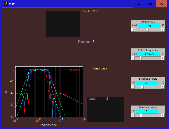
A second example (afiltS.m)

Now that we have covered most of the basic concepts and techniques, its time to explore the true power of plt by reviewing the design of a real GUI in one of the application areas that Matlab was designed for. The application I have chosen is the display and analysis of the classical analog filters. Granted this is not a particularly novel idea as it probably has been done before in Matlab and other languages, but nonetheless it serves various educational and practical needs and there is always room to apply our own slant to the project. I'll start with a relatively modest set of goals:
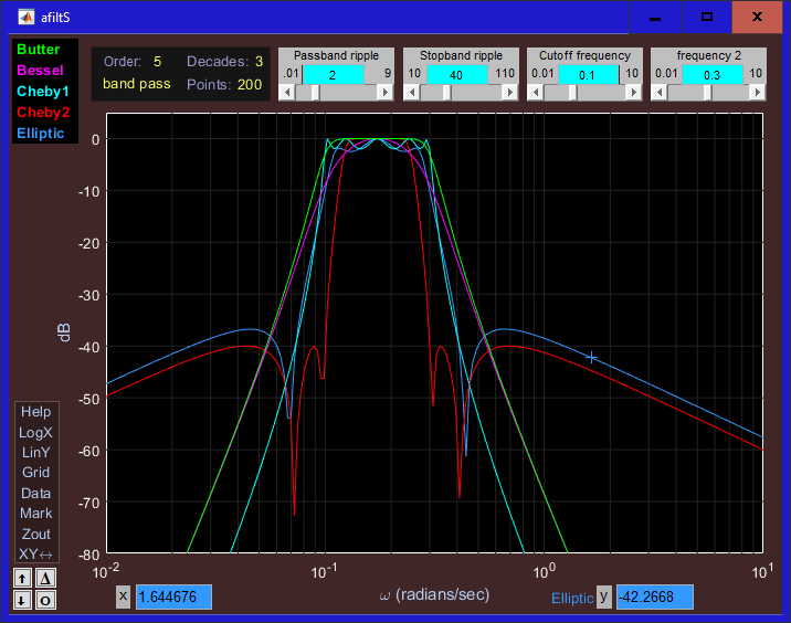
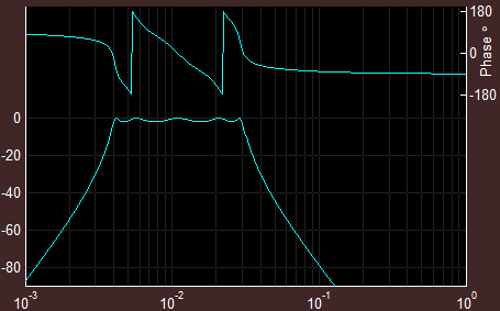
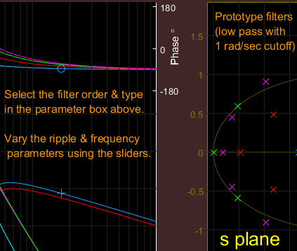
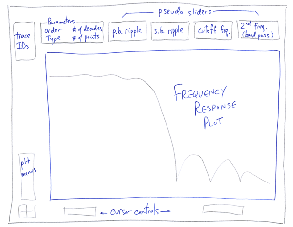
As is my habit, I start with a sketch to clarify my thoughts. I decide to use an array of four pseudo sliders along the top to control the continuously adjustable parameters (edge frequencies & ripple) The four remaining filter and display parameters are grouped to the left of the sliders inside a box for visual appeal and to allow those four parameters to be moved around as a group when repositioning. The Trace IDs to the left of that will be named after the classical filter types and be used to select which filters to display. The plot and the cursor controls and readouts along the bottom edge are the standard ones created by the plt pseudo object.

By the way, I've called this program afiltS.m (supplied in the demo folder) where the "S" stands for "Simplified" because it is a simplified version of afilt.m (also in the demo folder) which has several more advanced features. But of course, here we want to start simple.

Ok ... it's time to start writing code. First, we use the arrange function to initialize the positions of the 10 pseudo objects we will be creating. The next two lines define band and filter types to be plotted and the fourth line creates the first pseudo object (a plot) and assigns it a screen position of p{1}, the first position in the cell array created by the arrange function. Actually this object is a super pseudo object, including an axis, traces, axis labels, grid lines, and cursor controls (the last two being pseudo objects in their own right):
function afilt()
  p = arrange(10);
  band =   {'low pass' 'high pass' 'band pass' 'stop band'};
  ftypes = {'Butter'   'Bessel',   'Cheby1'    'Cheby2'      'Elliptic'};
  S.tr = plt(0,zeros(1,5),'TraceID',ftypes,'Options','logX','xy',p{1},...
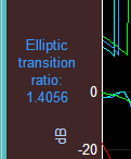
             'Ylim',[-80 5],'LabelX','\omega (radians/sec)','LabelY','dB');
Notice that we used plt's 'xy' parameter to position the plot within the figure window (although you will soon learn that this parameter can do far more than that). The data to be plotted for all 5 traces is defined in the plt call (as it must), but notice that each trace just contains the single point (0,0). When calling plt from the command line, you almost always include the actual plot data in the argument list, however in a GUI more often than not the data supplied is just a placeholder. The real data is loaded later (by the callback in this example). The callback will need to know where to put the plotting data, so the trace handles are saved in a 1x5 array called S.tr (the plt return value). In the code below, we will add the handles of the remaining pseudo objects to the S structure.

Next, we will define a frame (the box pseudo object), followed by four more pseudo objects (an edit object and three popups) that will be placed inside that frame:
  plt('box',            p{2}); % create a frame for the 4 filter parameters
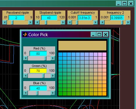
  S.n    = plt('edit',  p{3} ,[5 1 25],   @cb,'BackGr',[1 1 1]/12,'label','Ord~er:');
  S.band = plt('pop',   p{4} ,band,       @cb,'index',3,'swap');
  S.dec  = plt('pop',   p{5} ,1:5,        @cb,'index',3,'label','Decades:','hide');
  S.pts  = plt('pop',   p{6} ,50*2.^(1:5),@cb,'index',2,'label','Points:', 'hide');
Note that when you change any of these controls, the same callback function (cb) is executed. For more complicated interfaces you may want to have different callbacks for each control, but this one function suffices here. For the last popup, the choice vector could have been specified as [100 200 400 800 1600] but I chose to write it in terms of powers of 2. The [5 1 25] parameter of the pseudo edit object means that its initial value will be 5 with min/max limits of 1 and 25. The string 'Order' is used as a label for the edit object, but notice that there is a tilde character (~) inserted into that string. This is to change the amount of space (width) allocated to the label. You might want to experiment by moving and/or removing the tilde character to see how that affects the label width. 
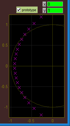
Notice that the first popup defined (S.band) includes the 'swap' parameter at the end of the call. The effect of that extra parameter is described in the
afilt section, where you can also learn other details about this application not discussed here.

And finally, let's finish off the main function by creating the last four pseudo objects (sliders):
  S.Rp   = plt('slider',p{7} ,[ 2  .01    9],'Passband ripple', @cb);
  S.Rs   = plt('slider',p{8} ,[ 40  10  110],'Stopband ripple', @cb);
  S.Wn   = plt('slider',p{9} ,[.1  .01   10],'Cutoff frequency',@cb,5,'%3.2f 6 2');
  S.Wm   = plt('slider',p{10},[.3  .01   10],'frequency 2',     @cb,5,'%3.2f 6 2');
  set(gcf,'user',S);  cb; % save parameters for cb, and initialize the plot
% end function afiltS
The [2 .01 9] on the first slider has the same meaning as the similar pseudo edit parameter mentioned above, i.e. 2 is the initial value with min/max limits of .01 and 9. The @cb specifies the callback function. For the last two sliders, there are two additional parameters after the callback. The first of these ("5") indicates that the slider will move logarithmically (so for example the slider will move the same number of pixels going from .01 to .1 as it does when changing from .1 to 1. The final parameter '%4.3f 6 2' is shorthand for '%4.3f %6v %2v' and specifies the display format for the min value, current value, and max value respectively. For more details about the parameters for these pseudo sliders consult the Pseudo objects section.

All we have left to do to finish the coding is to write the callback. We could choose to write a stub that merely returns, or perhaps displays a string on the command window, as we did some of the callbacks in the previous example. That way we could get on with the task of positioning the objects in the figure window. The advantage is that sometimes just moving these objects around makes us realize we have conceived them poorly and inspires us to go back to the drawing board. In this case, since the interface is pretty simple, let's go ahead and complete the callback. The comments in the code should be sufficient to understand how the callback works:
function cb() % callback function for all objects
  S = get(gcf,'user');  N = plt('edit',S.n);             % get handle list and filter order
  dec = plt('pop',S.dec);  pts = 50*2.^plt('pop',S.pts); % get # of decades and # of points
  bi = plt('pop',S.band);                                % get filter band index (low,high,band,stop)
  Wn  = plt('slider',S.Wn);  Wm = plt('slider',S.Wm);    % get filter frequency & frequency 2
  Rp  = plt('slider',S.Rp);  Rs = plt('slider',S.Rs);    % get passband and stopband ripple
  if bi>2 Wn = [Wn Wm]; v = 'visON'; else v = 'visOFF'; end;
  X = round(log10(mean(Wn)) - dec/2 + .5);  X = logspace(X,X+dec,pts); % X-axis (radians/sec)
  plt('slider',S.Wm,v);       % hide or show frequency 2
  af(bi,N,Wn,Rp,Rs,X,S.tr);   % compute frequency response & set trace data
  cur(-1,'xlim',X([1 end]));  % set Xaxis limits
%end function cb
The first six lines of the callback retrieve the parameters from every control. (We have to do this because cb doesn't know which control has been modified.) If we have selected low pass or high pass with the popup control (bi = 1 or 2) then we don't need the second frequency slider, so we turn it off ('visOFF'). If it is a bandpass or stopband filter (bi = 3 or 4) then we turn the second frequency slider on ('visON'). A lot happens in the next line, a for loop that sequences thru the five filter types (Butterworth, Bessel, Chebyshev types 1 and 2, and Elliptic), computing the frequency response by calling the af function and saving the results into the y coordinate of the respective trace. The last line sets the x-axis limits in case it was the number of points or the number of decades that had been modified.

Ok, after 27 lines of code we are done with the GUI design. The only remaining part is to write the af function which computes the frequency response of the five filter types. I won't discuss this function here since this is a purely computational function and does not add to our understanding of GUI programming (although this might be the most interesting part of the code for some).
Now when you type afiltS at the command prompt, you should see a figure similar to this. Although the program is essentially functional at this point, the haphazard arrangement of the controls makes that difficult to determine. So let's fix that now.

As with the previous example, we could allow the controls to be moved around by typing plt move into the command window, this time there is an easier way because we have included a plot in our design. Simply click on the red string plt move; that is in the upper right corner of the plot. You can tell that you are now in "move" mode because the pseudo sliders have been grayed out (as well as any uicontrols, although in this example there are none).

The "Order" control is far too tall, so start by shrinking that down to size using the right click and drag method. The gray box near the top is the frame, so move that to a spot resembling the sketch and then move the 4 controls inside it. When you get that frame as well as the 4 pseudo sliders positioned properly, you will have room to make the plot bigger, filling most of the figure area. After doing that you should click on the red "plt move;" again and you will notice that the TraceID box and the cursor controls now appear. (Initially, those elements were hidden because the plot was too small to allow room for them.). Then click on the red "plt move;" again to re-enable the move mode so you can make your final adjustments.

Once you get the 10 objects positioned as you want, as with the previous example, left-click once on every object in the order that they were created. As we are doing this, the text below will appear in the command window:
 xy:   1  .125 .105 .850 .760;  % axes
axi:  53  .108 .888 .228 .088;  % axes
edi: 211  .174 .936 .040 .030;  %   5  
pop: 102  .110 .718 .150 .200;  % band pass
pop: 103  .314 .756 .050 .200;  % 3
pop: 104  .290 .716 .080 .200;  % 200
sli: 401  .350 .946 .150     ;  % Passband ripple
sli: 406  .510 .946 .150     ;  % Stopband ripple
sli: 411  .670 .946 .150     ;  % Cutoff frequency
sli: 416  .830 .946 .150     ;  % frequency 2
Then as before, we copy and paste those lines into the beginning of the source code, remove the first two columns and add brackets so that the position arrays for a ten-element cell array. After editing the comments somewhat we have:

  p = {[.125 .105 .850 .760];  % plot    position
       [.108 .888 .228 .088];  % box     position: Parameter frame
       [.174 .936 .040 .030];  % edit    position: filter order
       [.110 .718 .150 .200];  % popup   position: filter band
       [.314 .756 .050 .200];  % popup   position: # of decades
       [.290 .716 .080 .200];  % popup   position: # of points
       [.350 .946 .150     ];  % slider  position: Passband ripple
       [.510 .946 .150     ];  % slider  position: Stopband ripple
       [.670 .946 .150     ];  % slider  position: Cutoff frequency
       [.830 .946 .150     ]}; % slider  position: frequency 2

After saving afiltS.m and then restarting the program, we should see something like this.

Notice the red text "plt move;" is no longer there in the corner of the plot window. (It appears only when the arrange function has been used to generate the positions.) But if you want to go back into positioning mode to make further adjustments (which will almost always happen) you can RIGHT click on the delta button near the lower left corner of the figure. (Or you can always type "plt move" in the command window.). RIGHT click on the delta button again to turn off the positioning mode and return to normal operation.

In this example, the 'xy' parameter in the plt command (line 4 of afiltS) included just a single array (p{1}) which specifies the position of the plotting axis. However the 'xy' parameter may include positions for other objects that are part of the plt super object, such as the TraceID box, the menu box, axis labels, and various cursor controls. (See the 'xy' command explained in the
Axis properties section.) The OID (object ID) described in that section is the number in the 2nd of the two columns that we removed from the text that we pasted in from the command window. For example, suppose we wanted to make the Y edit box wider. Change to position mode, and use the mouse to resize that object. When you release the mouse button you will see a line in the command window such as:
 xy: 206  .786 .006 .140 .047;
The "206" is the OID for the 'xy' parameter. If we add this row of 5 numbers (starting with the OID) to the xy parameter, then those coordinates will be used to position the Y edit box.

You can find more information about this simplified version (afiltS) as well as the more advanced version (afilt) discussed below in the afilt section.

Enhancing afiltS (creating afilt)

Play with afiltS for a while first to see that it behaves as you expect and then to see if you have any ideas for how you might enhance the program to make it more useful or pleasing to use. I came up with the seven enhancements below and after adding them to the code I renamed it to afilt.m. The original version afiltS.m is better for a gentle introduction to GUI design, but if you are interested in learning more following the coding of these seven enhancements below could be a could place to start.

1.) Adding a multi-line text string (elliptic transition ratio)

I was curious (mostly for the elliptic filter) how the width of the transition band (the space between the passband and the stopband) varied as the filter order changed as well as the four slider parameters. Could I define such a measure, figure out how to compute it and find a place on the GUI to display it?

For a low pass or passband filter, I characterized the transition width in terms of the ratio of these two frequencies:
        The frequency where the stop band spec is first achieved
        divided by the last frequency where the passband spec is still achieved
For a high pass or stopband filter, the ratio is:
        The frequency where the pass band spec is first achieved
        divided by the last frequency where the stopband spec is still achieved

I added an additional line to the position array at the beginning of the program, to define the location for the new text object. As with the other object positions, initially it was just a wild guess which was refined using the plt repositioning mode.

Once the transition ratio is calculated (saved in the variable h) it only takes this one line to convert it into a multi-line string:
set(S.etr,'string',prin('Elliptic ~, transition ~, ratio: ~, %5v',h));
Because the sprintf function does not handle cell arrays, this operation normally would require several awkward lines of code, but this is simplified by using the prin.m supplied in the plt folder. To see the full documentation for prin simply type prin with no arguments into the command window.

2.) Selecting colors

My second idea was to allow the user to control at least some aspect of the color choices used in the application. Actually, I don't think such a simple application like this really needs this flexibility, but my ulterior motive was to showcase the ColorPick pseudo object and how easy it is to add to your GUI and how easy it is to select the color you find most pleasing for any display element.

This was one of the simplest of the five enhancements requiring just the three extra lines shown below. I decided to enable color adjustment of five screen elements. The first four are the pseudo sliders at the top edge of the figure that control the pass and stop band ripple and the cutoff frequencies. The fifth element to gain this color adjustment feature is the multi-line text string (elliptic transition ratio) mentioned above. (It would be easy to extend this to other graphic elements.) In this figure, I have changed the background color of the sliders from its default gray to orange. I encourage you to play around with this ColorPick figure. (Just right-click on any of afilt's pseudo sliders or the multi-line text string to bring up ColorPick.) If you have ever dealt with the frustrations of assigning screen colors, I think you will be pleasantly surprised about how easy it can be. (Read about the details of the ColorPick object here:
Pseudo objects)

The first line (below) puts the handles of all the objects associated with pseudo sliders into "h". Then the 5th element of each slider is removed, since that is the edit box portion which generally is set to a contrasting color. The second line assigns the ColorPick object as the buttondown function (the right click action) to the 4 pseudo sliders as well as to the elliptic ratio text object. If we stopped there (i.e. omitted the third line) then we would be able to pick 16 different colors for the sliders (i.e 4 components for each of the 4 pseudo sliders). However, that's more flexibility than we probably would want and actually might be a nuisance. It's probably better to tie all 16 of those objects together so that when you change any one of them, the other 15 automatically change to agree with the new color. The third line accomplishes that by setting an application data variable as explained in the ColorPick Pseudo object documentation.
  h = plt('slider',S.sli,'get','obj'); h(:,5)=[]; h = h(:); 
  set([h; S.etr],'buttondown','plt ColorPick;'); 
  for k = 1:length(h) setappdata(h(k),'m',{'backgr' h}); end; 

3.) Adding the phase display


Since the phase of the frequency response is an important characteristic in some applications, I thought it would be useful to have the plot show phase as well as amplitude. So far we have only used the left-hand axis, so the easiest way to show the phase information is to plot it on the right-hand axis. Usually, the right-hand axis is used to superimpose traces on the left hand axis, although in this instance I decided it would be clearer to plot the phase above the magnitude so the traces would not overlap. That choice allows us to display both magnitude and phase for all five filter types at once without the display becoming hopelessly cluttered and confusing. This is accomplished by adjusting the left and right Yaxis limits so that the magnitude and phase traces don't overlap. The tick mark labels are set explicitly so that they only appear in the valid range of the display. Here is an example of what the display looks like when a single filter type (Cheby1) is enabled.

It would have been natural to expand the TraceID box to include 10 elements instead of 5 however that has the following drawback. To enable or disable the traces associated with a particular filter type (Cheyb1, for example) one would have to click on two traceID tags, one for the magnitude and one for the phase. That is somewhat unnatural and it would be less cumbersome to do this with just a single click. The trick to make this happen is to link traces 1 and 5 (Butterworth mag/phase) and to link traces 2 and 6 (Bessel mag/phase), etc. so that 5 is enabled only when trace 1 is enabled, etc. This linking can be done in a single line inside the callback function, and I will show that line in section 4 below since that enhancement also involves linking traces.

4.) Adding the pole/zero plot


The analog filters are designed by first designing a prototype filter (always low pass) and then transforming it as selected (high pass, stopband, passband) with the requested filter cutoff frequencies. Displaying the roots of the prototype filter in the s-plane can help our understanding of the design and use of the five filter types displayed by afilt. Alternatively, you may display the poles and zeros of the filter after it has been transformed by unchecking the prototype checkbox above the pole/zero plot.

I could have used plt's subplot parameter to create both plots (Mag/Phase plot on the left and Pole/Zero plot on the right all with a single call to plt. However because the characteristics of these two plots are so dramatically different, this would have been difficult and I decided to use a separate call to plt for each of the two plots. This necessitated using the Fig parameter on the second call so that both plots are created in the same figure window. Like the Mag/Phase plot on the left, the Pole/Zero plot uses 10 traces (the first 5 to display the zeros for the 5 filter types, and the next 5 to display the poles. Actually, an 11th trace was added to show a unit circle on the plot. A unit circle doesn't have the significance it does on z-plane plots, but it still provides a useful size reference, and some of the filter types have roots placed along or near the unit circle. Usually, the x/y cursor readout appears below the plot, but for this plot, they were moved to the top because that's where there was the most room (allowing for a bigger plot in a given figure size). If you enable only the Bessel filter traces, the figure will look like the one shown here. Note that the Bessel filter has only poles (X's on the plot) whereas some of the filter types will have both poles and zeros (X's and O's).

This single line was added to the callback function so that if you enabled or disabled the magnitude display of a certain filter type (Butterworth for example) then the associated phase trace, zeros trace and poles trace would also be appropriately enabled or disabled:
t = plt('show');  t = t(find(t<6));  plt('show',[t t+5 t+10 t+15 21]);
 % for traceID callback
t (using the find subscript) will contain a list of magnitude traces that are enabled, while t+5 will be a list of the associated phase traces, t+10 will be a list of the associated zeros traces, and t+15 will be a list of the associated poles traces. Trace 21 (showing the unit circle) is always enabled.

Often when the TraceID callback is a simple one or two-line function, it is more convenient to include the entire TraceID callback in the plt parameter list. Look at the function afiltALT.m (an alternate version of afilt also supplied in the demo folder) for an example of how this is done.

5.) Display of phase delay and group delay


Since the figure window is already becoming a bit crowded, I decided to display the phase delay and group delay in separate figure windows. LEFT clicking the button shown here above the prototype checkbox opens a new figure window showing the phase delay for all 5 filter types using all the currently selected parameters. This is essentially the phase response divided by the frequency at each point. RIGHT clicking the button opens yet another figure window showing the group delay for all 5 filter types. This is essentially the derivative of the phase response.

6.) Saving/restoring the GUI state using a configuration file

It would be nice if whenever we made a change to the figure size/position or the color selection, that these changes would be recorded so that the application looks the same the next time it is restarted. While we are at it, we might as well remember the state of the eight filter parameters (shown above the plot) so that on start up, the figure looks identical to the way it was when it was shut down. Also, we save the numerators and denominators of the s-plane polynomials for all 5 filter types that were used to generate the frequency response on the display when the figure was shut down.

To implement this, before the call to plt, let's choose a file name and path for saving the configuration data:

  S.cfg = [which(mfilename) 'at']; 

Next let's add a new function, called cfg which saves the current configuration to this file as a 11 element cell array:
function cfg() % write configuration file
  S = get(gcf,'user');  s = plt('slider',S.sli(1),'get','obj');
  cf = {plt('edit',S.n);    plt('pop',[S.band S.dec S.pts]);  plt('slider',S.sli);
        get(s(2),'backgr');  get(S.etr,'color');              get(gcf,'position')};
  num = get(S.tr(1),'user');  den = get(S.tr(2),'user');
  save(S.cfg,'cf','num','den');
Then right before we initialize the plot, we load the configuration file if it exists and set the GUI elements to agree with the data in the file:
  if exist(S.cfg) load(S.cfg);
                  % load configuration file if it exists -------------------
                  plt('edit',S.n,'value', cf{1});
                  plt('pop',[S.band S.dec S.pts],'index',num2cell(cf{2}));
                  plt('slider',S.sli,'set',num2cell(cf{3}));  set(h,'background',cf{4});
                  set(S.etr,'color',cf{5});                   set(gcf,'position',cf{6});
  end;
And finally we add this parameter to the plt call:

    'closeReq',@cfg 

This instructs plt to call the function that saves the configuration data when the user closes the figure window to exit the application.

7.) Adding temporary user help message

To define the help text shown in the figure below, these four lines were added to the beginning of the afilt routine:

htxt = {'Select the filter order & type' 'in the parameter box above.' '' ...
        'Vary the ripple & frequency' ' parameters using the sliders.' -1.28+.72i 2i ...
        's plane'  .4+.2i 'color' 'yellow' 'fontsize' 20 2i ...
        'Prototype filters' '(low pass with' '1 rad/sec cutoff)' .05+.98i};

This help text allows a new user of the program to get started without having to consult any help files or manuals. The most important consideration should be that the help messages are not distracting in any way to the user who is already familiar with the help information presented. The HelpText pseudo object is ideal for this task since it provides a mechanism for removing the messages once you start using the program.

Note that we have defined three help strings within the htxt cell array, each delimited by 2i (which actually may be any complex number).

The first of these strings consists of the 5 lines that appear inside the left-hand plot (the 3rd line is a blank line). The -1.28+.72i after those five lines indicates that the upper left corner of the 5-line help text should be positioned at x = -1.28 and y = .72 (in normalized coordinates relative to the pole/zero plot axis). Since no color was specified, the default helptext color was used (orange).

The second help string consists of just the one line "s plane" and is positioned at x = .4 and y = .2 (again in normalized coordinates in the pole/zero plot axis). A font size of 20 and a color (yellow) was specified for this string. (Note that instead of the string 'yellow' we could have used the traditional Matlab color triple vector ([1 1 0]) or the alternate vector form allowed in plt calls ([100 100 0]) or by the single number 010100 (the most compact way of specifying colors in plt parameters). These alternate ways of specifying colors are explained more completely at the top of the Colors help section.

Finally, the last help string consists of three lines that appear inside the pole-zero plot (again using the same reference frame for the xy position as the previous two help strings and again using the default orange help string color).

Then this line was added at the end of the afilt routine to make the help text visible on the screen:

plt('HelpText','on',htxt);  % show help text

And lastly, this line was added to the end of the callback function (cb):

plt('HelpText','off');

That line ensures that as soon as the user starts doing anything with the program, the HelpText will disappear so that it does not become a distraction.

All the extra features added to afilt expanded the code considerably from the simpler afiltS version and it now consists of 176 lines of code. If one were to code an application with all the same features using Matlab without the pseudo objects provided by plt, the source code would like span two or three times as much code, and probably even more than that if you chose some other programming language. (GUI programming is notorious for its complexity.)

This concludes our discussion of the afilt example. To further your education in GUI programming with plt, I recommend reviewing the applications in the sig and math folders. Most of them have a rich GUI design and use the various plt features in interesting ways. Many of them also involve moving plots, which will be especially helpful if that is something you need for an application you are creating.